Introduction

SAR images

Active acquisition systems (compared to optical ones).

• All weather
• All illuminations conditions
• Possibility to control band

Big data

Change detection issues

Detection problem

Determining places where a change has occured over the time series.

A place can be defined as:

• pixels indices
• spatial coordinates

The detection can be seen as:

• a binary mapping
• a continuous mapping

Binary versus continuous mapping

Pixel versus object detection

Supervised versus unsupervised detection (1/2)

A technique is defined as supervised when its application needs the use of labeled examples $\{(\mathbf{x}_i,y_i)\}_{i=1,\dots,N}$ called training samples to work. It is a two-step procedure.

First step: Training: find $\hat{\theta}=\mathrm{argmax}_\theta \, \frac{1}{N}\sum_{i=1}^N r(f(\mathbf{x}_i,\theta), \mathbf{y}_i)$

Second step: Testing

Supervised versus unsupervised detection (2/2)

A technique is defined as unsupervised when its application do not need any training sample. This is a one-step procedure.

Only testing:

What type of change ?

Measure of accuracy

Depend on the problem: classificaiton or distance problem

Classification problem: How many pixels have been accurately classified ?

\[ \mathrm{GD} = \frac{\text{number px well detected}}{\text{number total px to be detected}},\, \mathrm{FP} = \frac{\text{number px falsely detected}}{\text{number px with no change}} \]

Distance problem: How well the change dissociate from the no-change ?

$\rightarrow$ ROC curve

Questions to answer when designing
a change detection system:

Issues encountered in SAR images

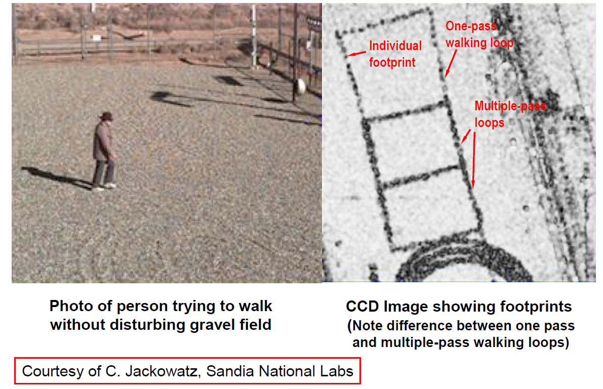
Co-registration

In order to detect change between several SAR acquistions, a co-registration phase has to be done.

Depending on the acquisition system (satellite vs plane), this phase can be difficult.

A poor co-registration will impact greatly the performance of change detection algorithms.

Speckle noise and pre-processing

Lack of training samples

A general framework for pixel-level methods

Illustration

Two steps:

Feature extraction (1/3)

First query: does the raw data allows to discern the changes we want to detect ?
$\rightarrow$If not, a transformation of the data is considered to be able to do it.

Raw data can be:

Feature extraction (2/3): Polarimetry based features

Polarimetry information consist in three complex values: $\mathbf{x} = [k_{HH}, k_{HV}, k_{VV}]^T$.

Several decompositions have been considered to retrieve physical behaviors of scatterers:

See: https://earth.esa.int/documents/653194/656796/Polarimetric_Decompositions.pdf for an onverview.

Feature extraction (3/3): Spectro-angular features

In high resolution SAR images, scatterers have dispersive and anisotropic behavior:

$\rightarrow$ Using wavelet decomposition, it is possible to retrieve this behaviour as a feature vector$^1$.

$^1$ A. Mian, J. Ovarlez, A. M. Atto and G. Ginolhac, "Design of New Wavelet Packets Adapted to High-Resolution SAR Images With an Application to Target Detection," in IEEE Transactions on Geoscience and Remote Sensing.

A brief glimpse into supervised methods (classification problem)

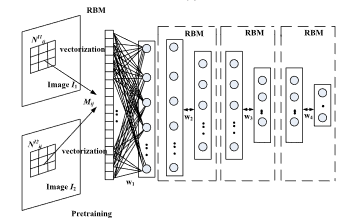
Deep learning methods

Recent works have started to try adapting deep learning methods from image processing litterature to SAR problems.

Most notable paper is:
M. Gong, J. Zhao, J. Liu, Q. Miao and L. Jiao, "Change Detection in Synthetic Aperture Radar Images Based on Deep Neural Networks," in IEEE Transactions on Neural Networks and Learning Systems, vol. 27, no. 1, pp. 125-138, Jan. 2016.

Pros: we can learn the type of change we want to detect if we have enough data.

Cons: amplitude, monovariate only and only bi-date + more validation needed (train and test on the same image?)

Semi-supervised classification

When there is not enough labeled data, we can turn to semi-supervised methods.

Idea: Idea: learn a classifier based on either geometrical constraints (SVM) or satistical ones (GMM for example).

One example:
L. Jia, M. Li, Y. Wu, P. Zhang, H. Chen and L. An, "Semisupervised SAR Image Change Detection Using a Cluster-Neighborhood Kernel," in IEEE Geoscience and Remote Sensing Letters, vol. 11, no. 8, pp. 1443-1447, Aug. 2014.

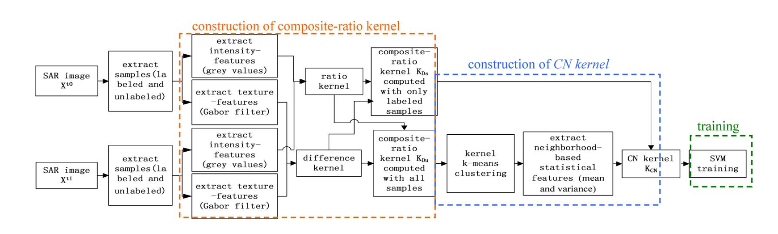
An overview of unsupervised methods at pixel-level

Post-classification (classification problem) (1/2)

Idea: After obtaining vectors, rather than measuring dissimilarities we can apply classic clustering algorithms (k-means, spectral clustering, EM). Then check for each pixel if the class has changed.

Post-classification (classification problem) (2/2)

Classification of SAR images has been considered in works such as:

Image rationing (distance problem)

Idea: Consider amplitude data for a pixel at date 1 $x_1$ and date 2 $x_2$. Since we know that the image is subject to speckle, consider the following distance:

The multiplicative nature of speckle is transformed to an additive one trough the $\log$ operator.

For example used in:
Y. Bazi, L. Bruzzone and F. Melgani, "Automatic identification of the number and values of decision thresholds in the log-ratio image for change detection in SAR images," in IEEE Geoscience and Remote Sensing Letters, vol. 3, no. 3, pp. 349-353, July 2006.

Coherent change detection (distance problem) (1/3)

Idea: Consider complex (amplitude + phase) data. Measure the coherence on a sliding windows between the two images.

On a window around the pixel, we have : $\left\{\begin{array}{c} I_1 = \left [ \begin{array}{cccc} x_1 & x_2 & ... & x_n \end{array} \right ] \in \mathbb{C}^N \\ I_2 = \left [ \begin{array}{cccc} y_1 & y_2 & ... & y_n \end{array}\right ] \in \mathbb{C}^N, \end{array}\right.$

The coherence is defined as follows: $d(I_1,I_2) = \frac{2|\sum_{k=1}^Nx_ky_k^*|}{\sum_{k=1}^N(|x_k|^2 + |y_k|^2)}$

$\rightarrow$ Allows to highlight fine changes in the phase between the acquisitions.

Coherent change detection (distance problem) (2/3)

Coherent change detection (distance problem) (3/3)

The approach was extended to multivaraite (polarimetric data) in:

Pros: Can find fine changes

Cons: Sensible to phase variation over time, bi-date, no thresold results.

Statistical based techniques (1/2): information theory techniques

Idea: Assign a probability model $p_\mathbf{x}(\mathbf{x})$ to the pixels. Then given the observed pixels, compare the distributions of data.

Comparing two distributions $p_1$, $p_2$: Kullback-Leibler divergence

Pros: Take into account the noise of the data, can be multivariate, some theoretical results to chose threshold.

Cons: Bi-date, sometimes given model no analytical expression of the divergence.

Used for example in:
A. D. C. Nascimento, A. C. Frery and R. J. Cintra, "Detecting Changes in Fully Polarimetric SAR Imagery With Statistical Information Theory," in IEEE Transactions on Geoscience and Remote Sensing, vol. 57, no. 3, pp. 1380-1392, March 2019.

Statistical based techniques (2/2): hypothesis testing techniques

Idea: Assign a parametric probability model $p_\mathbf{x}(\mathbf{x},\boldsymbol{\theta})$ to the pixels. Then test at each time if the parameters are equal (no change) or equal (change).

\[ \left\{ \begin{array}{ll} \mathrm{H}_{0}: & \boldsymbol{\theta}_{1} = \ldots = \boldsymbol{\theta}_{T} = \boldsymbol{\theta}_{0} \, ,\\ \mathrm{H}_{1}: & \exists (t, t'),\, \boldsymbol{\theta}_t \neq \boldsymbol{\theta}_{t'} \end{array}\right. \]

Pros: Multi-date, Take into account the noise of the data, can be multivariate, some theoretical results to chose threshold.

Cons: Sometimes given model difficult to obtain a decision function.

Example:
K. Conradsen, A. A. Nielsen, J. Schou and H. Skriver, "A test statistic in the complex Wishart distribution and its application to change detection in polarimetric SAR data," in IEEE Transactions on Geoscience and Remote Sensing, vol. 41, no. 1, pp. 4-19, Jan. 2003.

Detailing covariance based techniques

Description of the approach

We consider a sliding windows approach to consider spatially local data.

On this window, we assume i.i.d observations:

\[ \forall (k,t)\, \mathbf{x}_k^t \sim \mathbb{C}\mathcal{N}(\mathbf{0}_p, \mathbf{\Sigma}_t)\]

Idea: Compare the covariances $\mathbf{\Sigma}_t$ over time.

Why consider this methodology ?

Covariance equality testing under Gaussian context (1/3)

Denote by $\left\{\mathbf{X}_1,\dots,\mathbf{X}_T\right\}$ a collection of $T$ mutually independent samples of i.i.d $p$-dimensional complex vectors: $\mathbf{X}_t = [\mathbf{x}_1^{t},\dots,\mathbf{x}_{N}^{t}]$.

We assume $\forall (k,t),\,\mathbb{E}\{\mathbf{x}_k^{t}\}=\mathbf{0}_p$ and we denote $\mathbf{\Sigma}_t=\tau_t\boldsymbol{\xi}_t$ the shared covariance matrices among the elements of $\mathbf{X}_t$. $\boldsymbol{\xi}_t$ is the shape matrix ($Tr(\boldsymbol{\xi}_t) = p$) and $\tau_t$ is the scale.

Covariance equality testing under Gaussian context (2/3)

$^1$ D. Ciuonzo, V. Carotenuto and A. De Maio, "On Multiple Covariance Equality Testing with Application to SAR Change Detection," in IEEE Transactions on Signal Processing, vol. 65, no. 19, pp. 5078-5091, 1 Oct.1, 2017.

Covariance equality testing under Gaussian context (3/3)

Other approaches to compare covariance exists:

• Information theory$^1$
• Riemannian Geometry$^2$:

$^1$ A. D. C. Nascimento, A. C. Frery and R. J. Cintra, "Detecting Changes in Fully Polarimetric SAR Imagery With Statistical Information Theory," in IEEE Transactions on Geoscience and Remote Sensing, vol. 57, no. 3, pp. 1380-1392, March 2019.

$^2$ P.-A. Absil, R. Mahony, and R. Sepulchre, Optimization Algorithms on Matrix Manifolds

Non-Gaussianity high-resolution images

$^1$E. Ollila, D. E. Tyler, V. Koivunen and H. V. Poor, "Complex Elliptically Symmetric Distributions: Survey, New Results and Applications," in IEEE Transactions on Signal Processing, vol. 60, no. 11, pp. 5597-5625, Nov. 2012.

Covariance testing in the Compound-Gaussian model (1/2)

$^1$ A. Mian, G. Ginolhac, J. Ovarlez and A. M. Atto, "New Robust Statistics for Change Detection in Time Series of Multivariate SAR Images," in IEEE Transactions on Signal Processing, vol. 67, no. 2, pp. 520-534, 15 Jan.15, 2019.